"We introduce Stereo Anywhere, a novel stereo-matching framework that combines geometric constraints with robust priors from monocular depth Vision Foundation Models (VFMs). By elegantly coupling these complementary worlds through a dual-branch architecture, we seamlessly integrate stereo matching with learned contextual cues. Following this design, our framework introduces novel cost volume fusion mechanisms that effectively handle critical challenges such as textureless regions, occlusions, and non-Lambertian surfaces. Through our novel optical illusion dataset, MonoTrap, and extensive evaluation across multiple benchmarks, we demonstrate that our synthetic-only trained model achieves state-of-the-art results in zero-shot generalization, significantly outperforming existing solutions while showing remarkable robustness to challenging cases such as mirrors and transparencies."

1 - Problems

Stereo is a fundamental task that computes depth from a synchronized, rectified image pair by finding pixel correspondences to measure their horizontal offset (disparity). Due to its effectiveness and minimal hardware requirements, stereo has become prevalent in numerous applications. However, despite significant advances through deep learning, stereo models still face two main challenges:

1. Limited generalization across different scenarios: despite the initial success of synthetic datasets in enabling deep learning for stereo, their limited variety and simplified nature poorly reflect real-world complexity, and the scarcity of real training data further hinders the ability to handle heterogeneous scenarios;

2. Critical conditions that hinder matching or proper depth triangulation: large textureless regions common in indoor environments make pixel matching highly ambiguous, while occlusions and non-Lambertian surfaces violate the fundamental assumptions linking pixel correspondences to 3D geometry.

We argue that both challenges are rooted in the underlying limitations of stereo training data. Indeed, while data has scaled up to millions for several computer vision tasks, stereo datasets are still constrained in quantity and variety. This is particularly evident for non-Lambertian surfaces, which are severely underrepresented in existing datasets as their material properties prevent reliable depth measurements from active sensors (e.g. LiDAR).

In contrast, single-image depth estimation has recently witnessed a significant scale-up in data availability, reaching the order of millions of samples and enabling the emergence of Vision Foundation Models (VFMs). Since these models rely on contextual cues for depth estimation, they show better capability in handling textureless regions and non-Lambertian materials while being inherently immune to occlusions. Unfortunately, monocular depth estimation has its own limitations:

3. Its ill-posed nature leads to scale ambiguity and perspective illusion issues that stereo methods inherently overcome through well-established geometric multi-view constraints.

2 - Proposal

To address these challenges, we propose a novel stereo matching framework that combines the strengths of stereo and monocular depth estimation. Our model, Stereo Anywhere, leverages geometric constraints from stereo matching with robust priors from monocular depth Vision Foundation Models (VFMs). By elegantly coupling these complementary worlds through a dual-branch architecture, we seamlessly integrate stereo matching with learned contextual cues. In particular, following this desing, we can handle the aforementioned problems as follows:

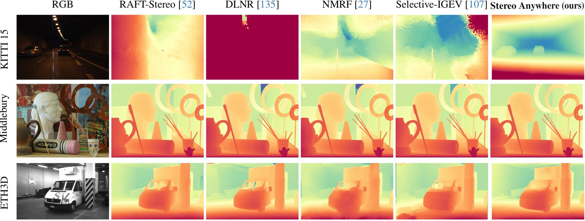
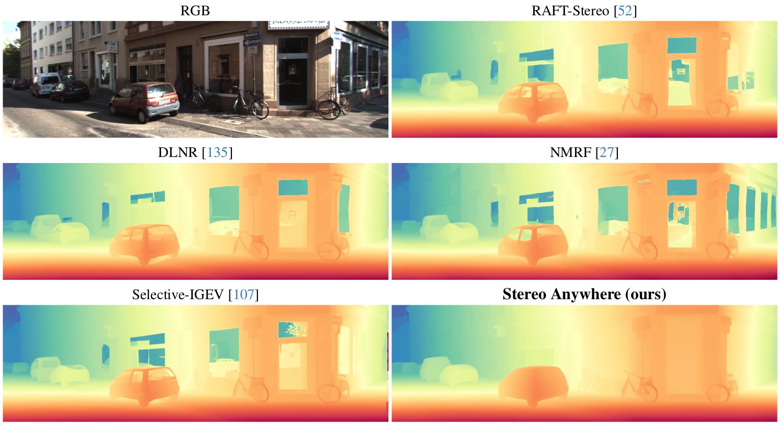
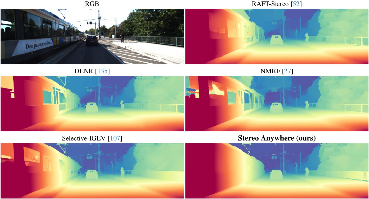
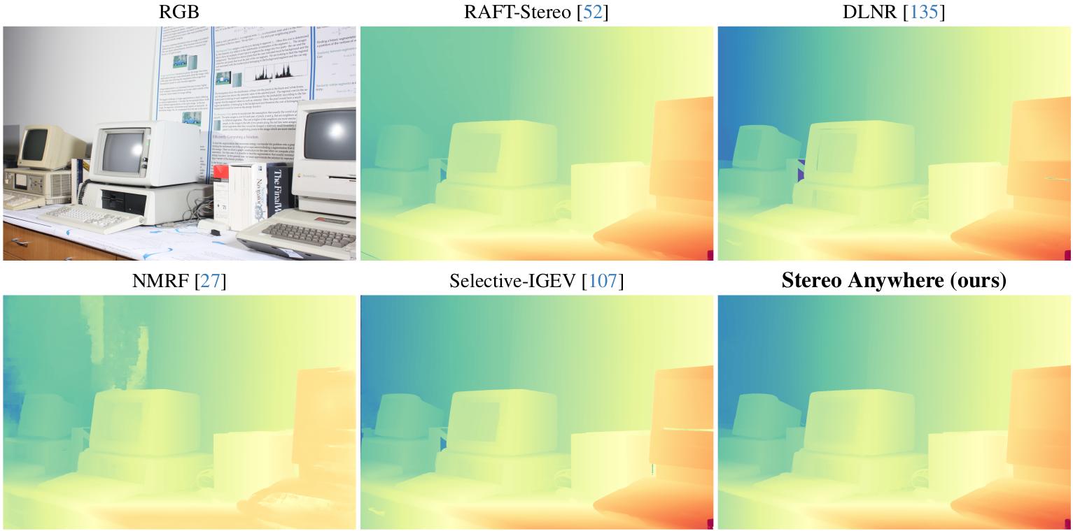
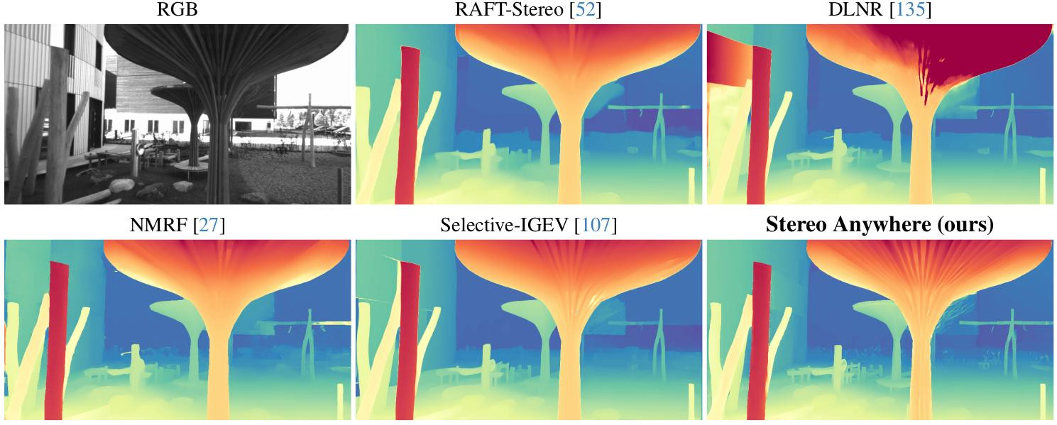
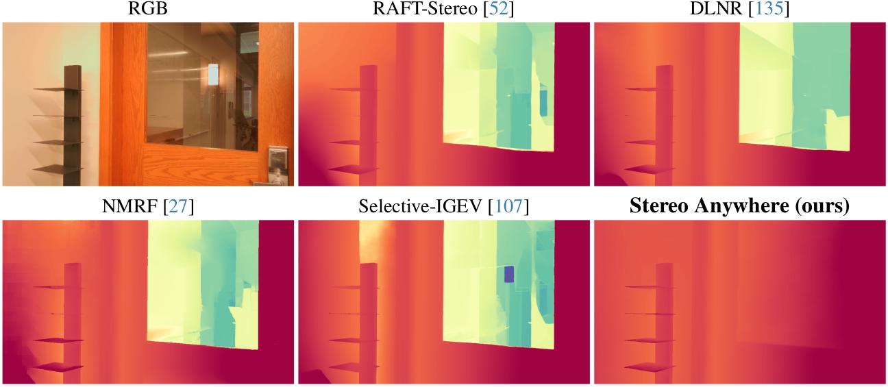
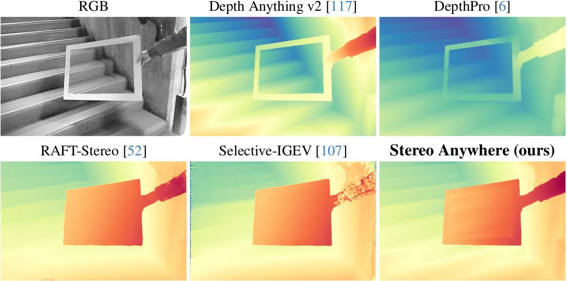
1. Zero-Shot Generalization: we show that by training on synthetic data only, our model achieves state-of-the-art results in zero-shot generalization, significantly outperforming existing solutions.

   Qualitative Results -- Zero-Shot Generalization. Predictions by state-of-the-art models and Stereo Anywhere.

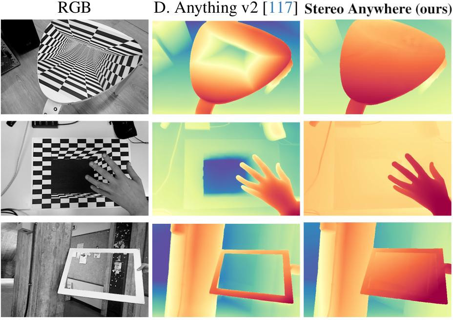
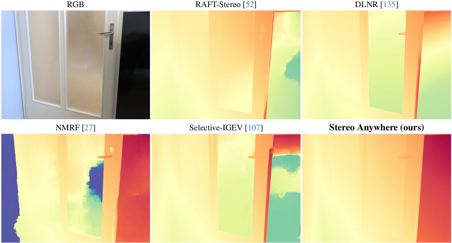
2. Robustness against critical conditions: we demonstrate that our model shows remarkable robustness to challenging cases such as mirrors and transparencies, as it leverages learned contextual cues from monocular depth Vision Foundation Models (VFMs).

   Qualitative results -- Zero-Shot non-Lambertian Generalization. Predictions by state-of-the-art models and Stereo Anywhere.

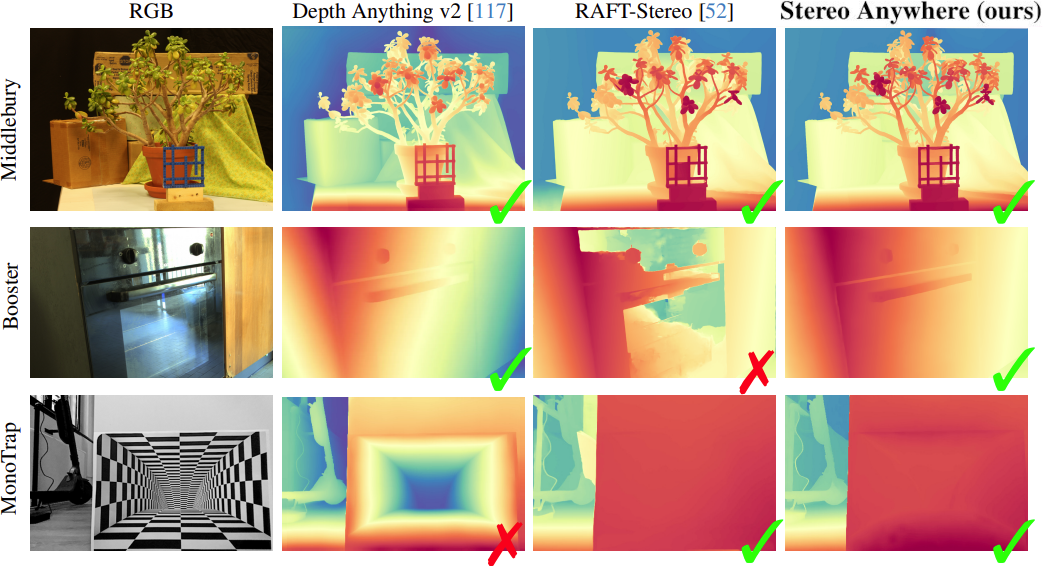
3. Robustness against monocular issues: we show that our model is immune to scale ambiguity and perspective illusion issues that plague monocular depth estimation, as it leverages well-established geometric multi-view constraints. We demonstrate this through our novel optical illusion dataset, MonoTrap.

   Qualitative results -- MonoTrap. Stereo Anywhere is not fooled by erroneous predictions by its monocular engine.

3 - Stereo Anywhere

Given a rectified stereo pair $\mathbf{I}_L, \mathbf{I}_R \in \mathbb{R}^{3 \times H \times W}$, we first obtain monocular depth estimates (MDEs) $\mathbf{M}_L, \mathbf{M}_R \in \mathbb{R}^{1 \times H \times W}$ using a generic VFM $\phi_M$ for monocular depth estimation. We aim to estimate a disparity map $\mathbf{D}=\phi_S(\mathbf{I}_L, \mathbf{I}_R, \mathbf{M}_L, \mathbf{M}_R)$, incorporating VFM priors to provide accurate results even under challenging conditions, such as texture-less areas, occlusions, and non-Lambertian surfaces. At the same time, our stereo network $\phi_S$ is designed to avoid depth estimation errors that could arise from relying solely on contextual cues, which can be ambiguous, like in the presence of visual illusions. Following recent advances in iterative models, Stereo Anywhere comprises three main stages, as shown in the following figure: I) Feature Extraction, II) Correlation Pyramids Building, and III) Iterative Disparity Estimation.

1. Feature Extraction. We extract image features from a frozen, pre-trained encoder applied to the stereo pair, producing feature maps $\mathbf{F}_L, \mathbf{F}_R \in \mathbb{R}^{D \times \frac{H}{4} \times \frac{W}{4}}$ for building a stereo correlation volume at quarter resolution. Context features are extracted from a similar encoder trained on monocular depth maps, leveraging strong geometry priors.

2. Correlation Pyramids Building. The cost volume is the data structure econding the similarity between pixels across the two images. Our model employs correlation pyramids -- yet in a different manner. Indeed, Stereo Anywhere builds two cost volumes: a stereo correlation volume starting from $\mathbf{I}_L, \mathbf{I}_R$ for image similarities and a monocular correlation volume from $\mathbf{M}_L, \mathbf{M}_R$ to encode geometric similarities -- (2) and (4). Unlike the former, the latter is robust to non-Lambertian surfaces, assuming a reliable $\phi_M$.

   1. Stereo Correlation Volume. Given $\mathbf{F}_L, \mathbf{F}_R$, we construct a 3D correlation volume $\mathbf{V}_S$ using dot product between feature maps: $$(\mathbf{V}_S)_{ijk} = \sum_{h} (\mathbf{F}_L)_{hij} \cdot (\mathbf{F}_R)_{hik}, \ \mathbf{V}_S \in \mathbb{R}^{\frac{H}{4} \times \frac{W}{4} \times \frac{W}{4}}$$

   2. Mononocular Correlation Volume. Given $\mathbf{M}_L, \mathbf{M}_R$, we downsample them to 1/4, compute their normals $\nabla_L, \nabla_R$, and construct a 3D correlation volume $\mathbf{V}_M$ using dot product between normal maps: $$(\mathbf{V}_M)_{ijk} = \sum_{h} (\nabla_L)_{hij} \cdot (\nabla_R)_{hik}, \ \mathbf{V}_M \in \mathbb{R}^{\frac{H}{4} \times \frac{W}{4} \times \frac{W}{4}}$$ Next, we insert a 3D Convolutional Regularization module $\phi_A$ to aggregate ${\mathbf{V}_M}$. We propose an adapted version of CoEx correlation volume excitation that exploits both views. The resulting feature volumes ${\mathbf{V}'}_M \in \mathbb{R}^{F \times \frac{H}{4} \times \frac{W}{4} \times \frac{W}{4}}$ are fed to two different shallow 3D conv layers $\phi_D$ and $\phi_C$ to obtain two aggregated volumes $\mathbf{V}^D_M = \phi_D({\mathbf{V}'}_M)$ and $\mathbf{V}^C_M = \phi_C({\mathbf{V}'}_M)$ with $\mathbf{V}^D_M,\mathbf{V}^C_M \in \mathbb{R}^{\frac{H}{4} \times \frac{W}{4} \times \frac{W}{4}}$.

   3. Differentiable Monocular Scaling. Volume $\mathbf{V}^D_M$ will be used not only as a monocular guide for the iterative refinement unit but also to estimate the coarse disparity maps $\hat{\mathbf{D}}_L$ $\hat{\mathbf{D}}_R$, while $\mathbf{V}^C_M$ is used to estimate confidence maps $\hat{\mathbf{C}}_L$ $\hat{\mathbf{C}}_R$: those maps are used to scale both $\mathbf{M}_L$ and $\mathbf{M}_R$ -- (5).

      To estimate disparities we can use a softargmax operator and the relationship between disparity and correlation: $$(\hat{\mathbf{D}}_L)_{ij} = j - \sum_{d}^{\frac{W}{4}} d \cdot \frac{e^{(\mathbf{V}^D_M)_{ijd}}}{\sum_{f}^{\frac{W}{4}} e^{(\mathbf{V}^D_M)_{ijf}}} \quad (\hat{\mathbf{D}}_R)_{ik} = \sum_{d}^{\frac{W}{4}} d \cdot \frac{e^{(\mathbf{V}^D_M)_{idk}}}{\sum_{f}^{\frac{W}{4}} e^{(\mathbf{V}^D_M)_{ifk}}} - k$$

      We also aim to estimate a pair of confidence maps $\hat{\mathbf{C}}_L, \hat{\mathbf{C}}_R \in [0,1]^{H \times W}$ to classify outliers and perform a robust scaling. Inspired by information entropy, we estimate the chaos inside correlation curves: clear monomodal-like cost curve -- the ones with low entropy -- are reliable -- while chaotic curves -- the ones with high entropy -- are uncertain. $$(\hat{\mathbf{C}}_L)_{ij} = 1 + \frac{\sum_{d}^{\frac{W}{4}} \frac{e^{(\mathbf{V}^C_M)_{ijd}}}{\sum_{f}^{\frac{W}{4}} e^{(\mathbf{V}^C_M)_{ijf}}} \cdot \log_2 \left( \frac{e^{(\mathbf{V}^C_M)_{ijd}}}{\sum_{f}^{\frac{W}{4}} e^{(\mathbf{V}^C_M)_{ijf}}} \right)}{\log_2(\frac{W}{4})} \quad (\hat{\mathbf{C}}_R)_{ik} = 1 + \frac{\sum_{d}^{\frac{W}{4}} \frac{e^{(\mathbf{V}^C_M)_{idk}}}{\sum_{f}^{\frac{W}{4}} e^{(\mathbf{V}^C_M)_{ifk}}} \cdot \log_2 \left( \frac{e^{(\mathbf{V}^C_M)_{idk}}}{\sum_{f}^{\frac{W}{4}} e^{(\mathbf{V}^C_M)_{ifk}}} \right)}{\log_2(\frac{W}{4})}$$

      To further reduce outliers, we mask out from $\hat{\mathbf{C}}_L$ and $\hat{\mathbf{C}}_R$ occluded pixels using a SoftLRC operator: $$\text{softLRC}_L(\mathbf{D},\mathbf{D}_R) = \frac{\log\left(1+\exp\left(T_\text{LRC}-\left| \mathbf{D}_L - \mathcal{W}_L(\mathbf{D}_L,\mathbf{D}_R) \right|\right)\right)}{\log(1+\exp(T_\text{LRC}))}$$ where $T_\text{LRC}=1$ is the LRC threshold and $\mathcal{W}_L(\mathbf{D}_L,\mathbf{D}_R)$ is the warping operator that uses the left disparity $\mathbf{D}_L$ to warp the right disparity $\mathbf{D}_R$ into the left view.

      Finally, we can estimate the scale $\hat{s}$ and shift $\hat{t}$ using a differentiable weighted least-square approach: $$\min_{\hat{s}, \hat{t}} \left\lVert \sqrt{\hat{\mathbf{C}}_L}\odot\left[\left(\hat{s}\mathbf{M}_L + \hat{t}\right) - \hat{\mathbf{D}}_L \right] \right\rVert_F + \left\lVert \sqrt{\hat{\mathbf{C}}_R}\odot\left[\left(\hat{s}\mathbf{M}_R + \hat{t}\right) - \hat{\mathbf{D}}_R \right] \right\rVert_F$$ where $\lVert\cdot\rVert_F$ denotes the Frobenius norm and $\odot$ denotes the element-wise product.

      Using the scaling coefficients, we obtain two disparity maps $\hat{\mathbf{M}}_L$, $\hat{\mathbf{M}}_R$: $$\hat{\mathbf{M}}_L = \hat{s}\mathbf{M}_L + \hat{t},\ \hat{\mathbf{M}}_R = \hat{s}\mathbf{M}_R + \hat{t}$$ It is crucial to optimize both left and right scaling jointly to obtain consistency between $\hat{\mathbf{M}}_L$ and $\hat{\mathbf{M}}_R$.

   4. Volume Augmentations. Volume augmentations are necessary when the training set -- e.g., Sceneflow -- does not model particularly complex scenarios where a VFM could be useful, for example, when experiencing non-Lambertian surfaces. Without any augmentation of this kind, the stereo network would simply overlook the additional information from the monocular branch. Hence, we propose three volume augmentations and a monocular augmentation to overcome this issue:

      • Volume Rolling: non-Lambertian surfaces such as mirrors and glasses violate the geometry constraints, leading to a high matching peak in a wrong disparity bin. This augmentation emulates this behavior by shifting some among the matching peaks to a random position: consequentially, Stereo Anywhere learns to retrieve the correct peak from the other branch.

      • Volume Noising and Volume Zeroing: we introduce noise and false peaks into the correlation volume to simulate scenarios with texture-less regions, repeating patterns, and occlusions.

      • Perfect Monocular Estimation: instead of acting inside the correlation volumes, we can substitute the prediction of the VFM with a perfect monocular map -- the ground truth normalized between $[0,1]$. This perfect prediction is noise-free and therefore the monocular branch of Stereo Anywhere will likely gain importance during the training process.

   5. Volume Truncation. To further help Stereo Anywhere to handle mirror surfaces, we introduce a hand-crafted volume truncation operation on ${\mathbf{V}}_S$. Firstly, we extract left confidence $\mathbf{C}_M=\text{softLRC}_L(\hat{\mathbf{M}}_L, \hat{\mathbf{M}}_R)$ to classify reliable monocular predictions. Then, we create a truncate mask $\mathbf{T} \in [0,1]^{\frac{H}{4} \times \frac{W}{4}}$ using the following logic condition: $$(\mathbf{T})_{ij}=\left[\left((\hat{\mathbf{M}}_L)_{ij} >(\hat{\mathbf{D}}_L)_{ij}\right) \land (\mathbf{C}_M)_{ij} \right] \lor \left[ (\mathbf{C}_M)_{ij} \land \neg(\hat{\mathbf{C}}_L)_{ij} \right]$$ The rationale is that stereo predicts farther depths on mirror surfaces: the mirror is perceived as a window on a new environment, specular to the real one. Finally, for values of $\mathbf{T}>T_\text{m}=0.98$, we truncate ${\mathbf{V}_S}$ using a sigmoid curve centered at the correlation value predicted by $\hat{\mathbf{M}}_L$ -- i.e., the real disparity of mirror surfaces -- preserving only the stereo correlation curve that does not "pierce" the mirror region.

      Qualitative Results - Volume Truncation. While Stereo Anywhere alone cannot entirely restore the surface of the mirror starting from the priors provided by the VFM, applying cost volume truncation allows for predicting a much smoother and consistent surface.

3. Iterative Disparity Estimation. We aim to estimate a series of refined disparity maps $\{\mathbf{D}^1=\hat{\mathbf{M}}_L, \mathbf{D}^2,\dots\,\mathbf{D}^l,\dots\}$ exploiting the guidance from both stereo and mono branches. Starting from the Multi-GRU update operator we introduce a second lookup operator that extracts correlation features $\mathbf{G}_M$ from the additional volume $\mathbf{V}^D_M$ -- (7). The two sets of correlation features from $\mathbf{G}_S$ and $\mathbf{G}_M$ are processed by the same two-layer encoder and concatenated with features derived from the current disparity estimation $\mathbf{D}^l$. This concatenation is further processed by a 2D conv layer, and then by the ConvGRU operator. We inherit the convex upsampling module to upsample final disparity to full resolution.

The figure above shows qualitative results on the KITTI 2012 dataset. We can notice how any existing stereo model is unable to properly perceive the presence of transparent surfaces, as in correspondence of the windows on buildings and cars. On the contrary Stereo Anywhere, driven by the priors injected through the VFM, properly predicts the disparity corresponding to the transparent surfaces.

The qualitative above shows qualitative results on the KITTI 2015 dataset, showing underexposed and transparent regions. While existing stereo networks struggle at dealing with both, Stereo Anywhere exposes unprecedented robustness.

The upper figure reports the Vintage scene from Middlebury 2014 dataset. Stereo Anywhere can properly estimate the disparity for the displays, where existing methods are fooled and predict holes.

The image above shows qualitative results on the ETH3D dataset -- Playground1. Once again, Stereo Anywhere proves its supremacy at predicting fine details such as branches and poles.

The upper figure reports a scene from Booster dataset, confirming how Stereo Anywhere can exploit the strong priors provided by the VFM to properly perceive the glass surface on the door, as well as challenging, untextured black surfaces of the TV appearing on the right.

The qualitative above showcases an image from the LayeredFlow dataset, highlighting once again the inability of the state-of-the-art networks to model transparent surfaces as those in the door, conversely to Stereo Anywhere which can properly identify their presence.

To conclude, this last figure collects a scene from our novel MonoTrap dataset. In this case, we report predictions by both state-of-the-art monocular and stereo models, as well as by Stereo Anywhere. The perspective illusions fooling monocular methods, unsurprisingly, do not affect stereo networks, which however lack in details. Stereo Anywhere effectively combines the strength of both worlds, while being not affected by any of their weaknesses.